7. Predator and prey
Competition and mutualism can be understood without much attention to the sizes of the species involved. But predation is quite different. Think of a producer, the prey, and a consumer, the predator. When the consumer is extremely large and the producer very small, as with a whale and krill, the relationship is called filter feeding. There the predator kills the prey. When the producer and consumer are roughly matched in size, they are called predators and prey. When the producer is much smaller than the consumer, but still independently mobile, the relationship is called parasitism. And when the consumer is much smaller still, and has difficulty moving around on its own, the relationship is called infection and disease. Symptoms of disease are part of the ecology of disease. In parasitism and disease, the consumer often does not kill the producer.
7.1. Further examples of predation
Amazing mechanisms for both capturing prey and avoiding predators have been discovered through evolution. Fulmar chicks,*, for example, can direct “projectile vomit” at predators approaching the nest too closely (Figure 12.1[fig_12_1]). This is not just icky for the predator. By damaging the waterproofing of an avian predator’s feathers, this ultimately can kill the predator. The chick’s projectile vomit is thus a lethal weapon.
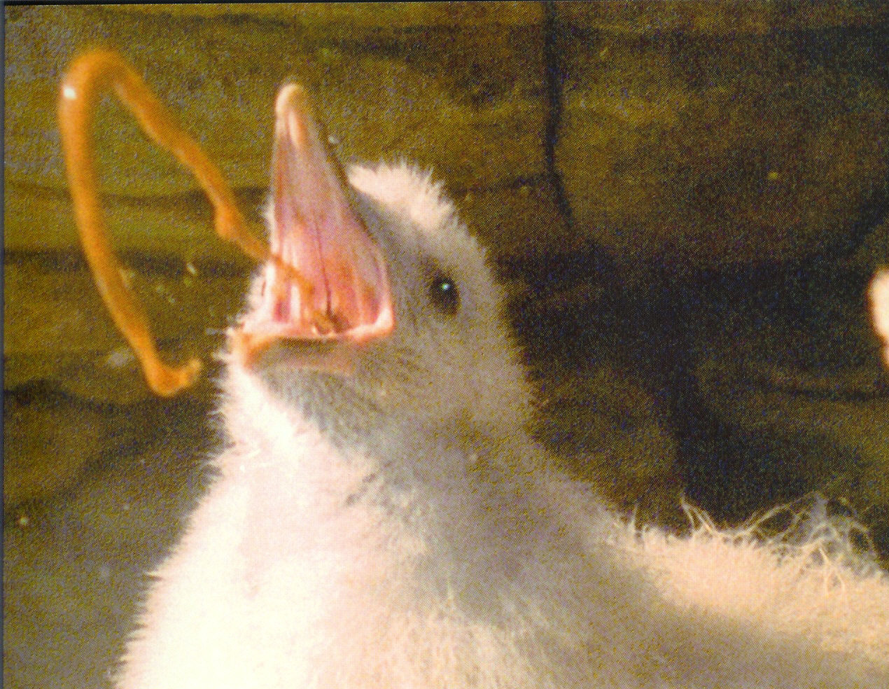
Fig. 7.1 Fulmer chick with projectile vomit as predator defense.
One of the most remarkable predatory weapons is that of pistol shrimp (Figure 12.2[fig12_2]). These shrimp have one special claw adapted to cavitation, and are capable of shooting bullets at their prey; colonies of these shrimp are loud from the sound of these bullets. But where does an underwater crustacean get bullets? Actually, it creates them from nothing at all—from cavitation. If you’ve ever piloted a powerful motorboat and pushed the throttle too hard, or watched a pilot do so, you’ve seen the propellers start kicking out bubbles, which look like air bubbles. But the propellers are well below the water line, where there is no air. The propellers are in fact creating bubbles of vacuum—separating the water so instantly that there is nothing left in between, except perhaps very low density water vapor. Such bubbles collapse back with numerous blasts, each so powerful that it rips off pieces of bronze off the propeller itself, leaving a rough surface that is the telltale sign of cavitation.
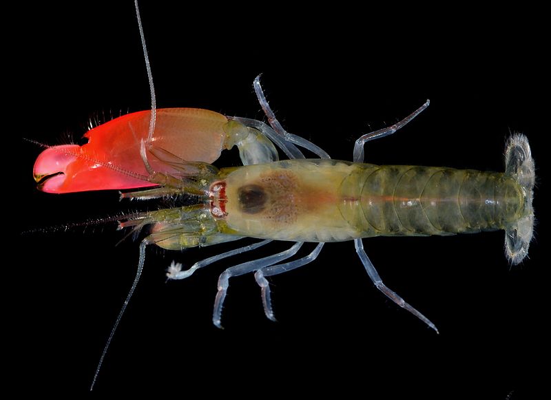
Fig. 7.2 Pistol-packing shrimp shoot cavitation bullets.
A pistol shrimp snap its pistol claw together so quickly that it creates a vacuum where water used to be. With the right circulation of water around the vacuum bubble, the bubble can move, and a shrimp can actually project its bullet of vacuum toward its prey. When the bubble collapses, the effect is like thunder attending a lightning bolt, when air snaps together after the lightning has created a column of near-vacuum (NatGeo video[https://www.youtube.com/watch?v=KkY_mSwboMQ]). But the consequences are quite different in water. While a loud sound might hurt the ears of a terrestrial animal, the sound does not rip apart the fabric of the animal’s body. This is, however, what intense sounds in water can do, traveling through water and through the water-filled bodies of animals. In effect, pistol shrimp shoot bullets that explode near their prey and numb them into immobility. Somehow evolution discovered and perfected this amazing mechanism!
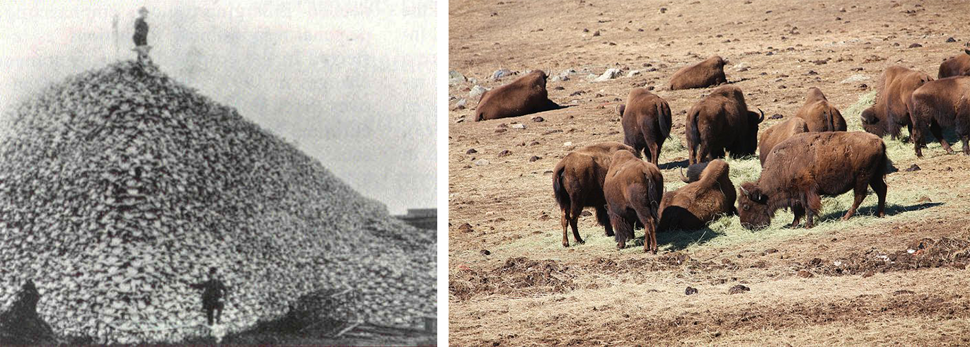
Fig. 7.3 Rifle-carrying humans shoot lead bullets—bison bones and remnant herd.
The ultimate weapons of predation, however, are those of our own species. Figure 12.3[fig12_3] (right) shows a remnant bison herd, a few hundred of the hundreds of millions of bison that migrated the plains not many generations ago. No matter how vast their numbers, they were no match for gunpowder and lead bullets, and they dropped to near extinction by the beginning of the twentieth century. The image at the left illustrates the epic efficiency of lead bullets by showing a nineteenth-century pile of bison bones, with members of the predator species positioned atop and aside.
7.2. Ecological communities are complex
Before proceeding with simplified models of predation, we want to stress that ecological communities are complex (Figure FigFoodWebMitchell). Fortunately, progress in understanding them comes piece by piece. Complex food webs, like the one illustrated in the figure, can be examined in simpler “motifs.”
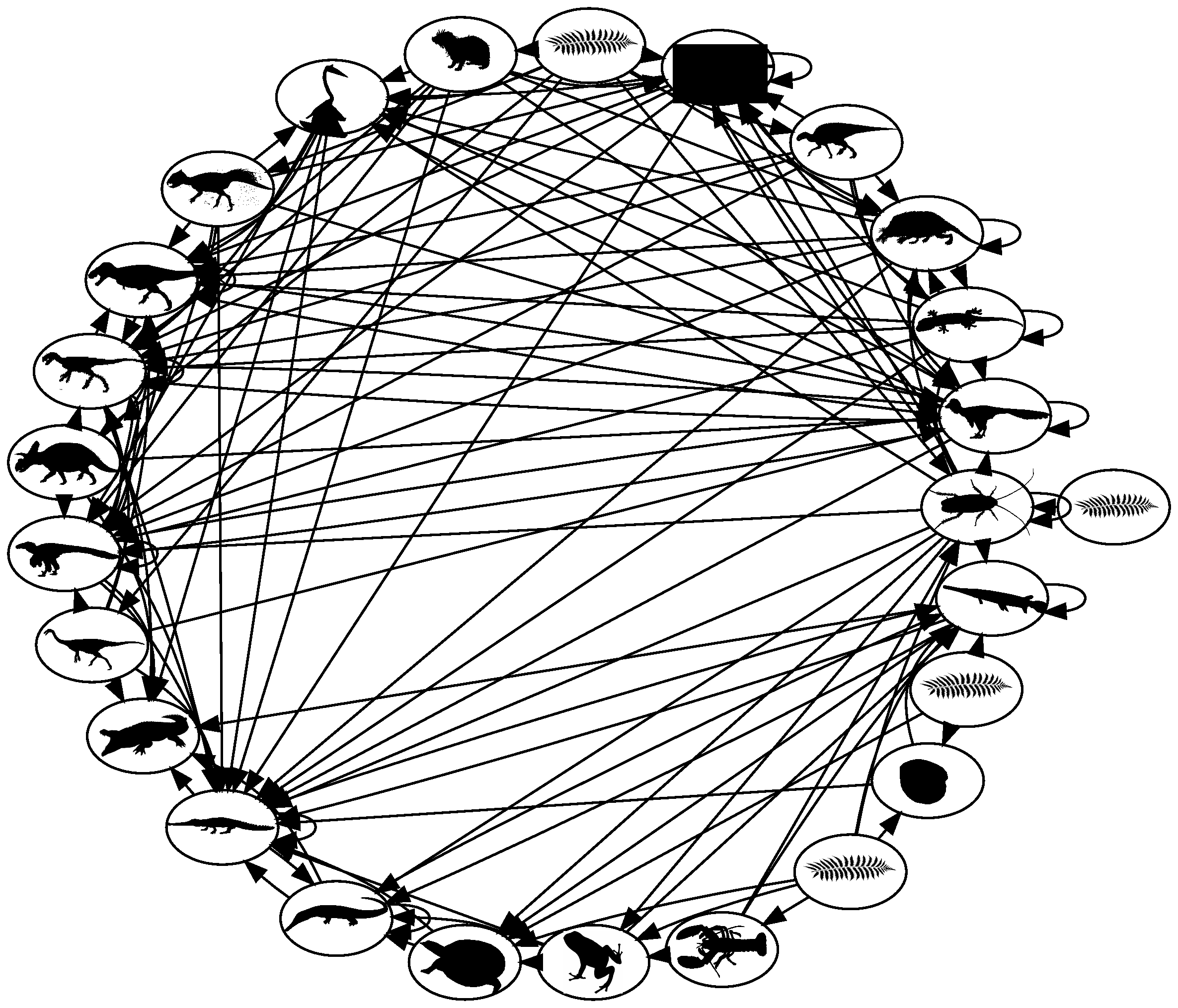
Fig. 7.4 Cretaceous terrestrial food web, Mitchell et al. 2012 PNAS.
You have seen in earlier chapters that there are two motifs for a single
Species: logistic and orthologistic, with exponential growth forming a fine
dividing line between them.
And in the prior chapter, you saw three motifs for two species:
predation, competition, and mutualism. 
Later you will see that there are exactly forty distinct three-species motifs,
one of which is two prey pursued by one predator. This is called “apparent
competition” because it has properties of competition.
7.3. Predator–prey model
For the next several chapters we will consider two species, starting with one predator and one prey. Figure FigPredPreyA depicts this situation, with one line sloping down and the other up.
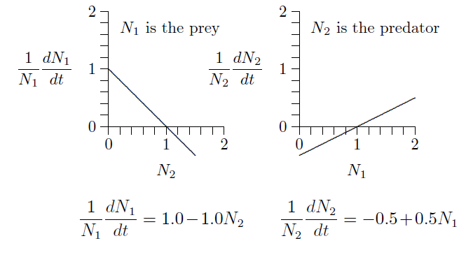
Fig. 7.5 Predator{prey interactions with corresponding equations.
The graph on the left describes the prey, because its numbers \(N_1\) are reduced when the numbers of predator, \(N_2\), increase. Likewise, the graph on the right describes the predator, because its numbers, \(N_2\), increase with the density of its prey, \(N_1\). The equations of growth are revealed by the slopes and intercepts of the two lines.
Since these are both straight lines, \(y=mx+b\), the equations can be written down simply from the geometry. The intercept on the left is \(+1\) and the slope is \(-1\). The intercept on the right is \(-1/2\) and its slope is \(+1/2\). The equivalent equations of the two lines appear below the graphs.
These specific equations can be generalized using symbols in place of actual numbers, writing \(r_1\), \(s_{1,2}\), \(r_2\), and \(s_{2,1}\) for the intercept \(+1.0\) and slope \(-1.0\) on the left and the intercept \(-0.5\) and slope \(+0.5\) on the right, as follows.
Merely by writing down the form of these geometric graphs, the classic Lotka–Volterra predator–prey equations have appeared:
Here is how the equations look in many textbooks, with \(V\) for prey density and \(P\) for predator density:
Volterra* arrived at the equation rather differently than we did, with a growth rate \(r\) for the prey, reduced by a rate \(\alpha\) for each encounter between predator and prey, \(V\!\cdot\!P\), and with a natural death rate \(q\) for predators and compensatory growth rate \(\beta\) for each encounter, \(V\!\cdot\!P\), between predator and prey.
To see the equivalence, divide the first equation through by \(V\) and the second by \(P\), then set \(V=N_1\), \(P=N_2\), \(r=r_1\), \(q=-r_2\), \(\alpha=-s_{1,2}\), \(\beta=s_{2,1}\). The Lotka–Volterra formulation will be revealed to be just the \(r+sN\) equations in disguise.
Figure 12.5[fig12_5] exposes the basic predator–prey equations from geometry, which reveal the unity of the equations of ecology, as you saw in Equation 5.2 (Ch 5). That analysis revealed a form of one-dimensional equation not considered in ecological textbooks—the orthologistic equation—and which is needed for understanding human and other rapidly growing populations.
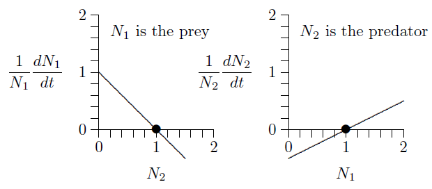
Now analyze these equations a bit. Suppose predator and prey densities are both 1, say 1 individual per hectare (\(N_1=N_2=1\)). Substitute 1 for both \(N_1\) and \(N_2\). What are the growth rates?
The population growth is zero for both species, so the populations do not change. This is an equilibrium.
This can be seen in the graphs below. The fact that both growth rates, \(1/N_1\,dN_1/dt\) and \(1/N_1\,dN_2/dt\), cross the horizontal axis at \(N_1=N_2=1\) (position of the dots) means that growth stops for both. This is called an equilibrium, a steady state, or, sometimes, a fixed point.
But what will happen if both populations are 2, say 2 individuals per hectare?
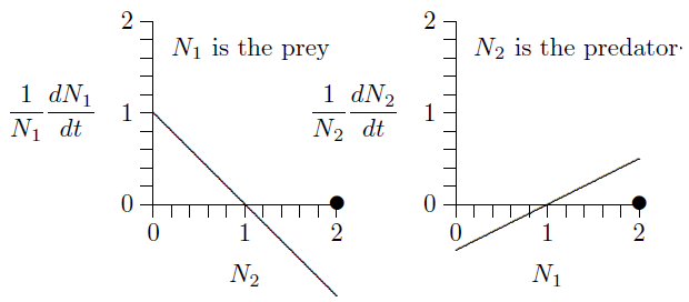
The prey growth rate, \(1/N_1\,dN_1/dt\), is negative at \(N_2=2\) (the line is below the horizontal axis) and the predator growth rate, \(1/N_1\,dN_2/dt\), is positive at \(N_1=2\) (the line is above the horizontal axis). So the prey population will decrease and the predator population will increase. Exactly how the populations will develop over time can be worked out by putting these parameters into the program in Chapter 8.2. Here it what it shows.